In this project we study the
evolution of charged droplets of a conducting viscous liquid.
The flow is driven by electrostatic repulsion (which pulls the
droplet apart) and capillarity (that stabilizes the droplet).
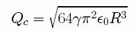
Charged droplets are known to be linearly unstable when the
electric charge Q is above the Rayleigh critical value.
Here we investigate the nonlinear evolution that develops
after the linear regime. Using a boundary elements numerical
method, we found that a perturbed sphere with critical charge
evolves into a fusiform shape with conical tips at time T, and
that the velocity at the tips blows up as (T-t)^alpha, with
alpha close to -1/2. In the neighborhood of the singularity, the
shape of the surface is self-similar, and the asymptotic angle
of the tips is smaller than the opening angle in Taylor cones.
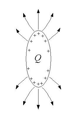
The figure above depicts a
charged conducting droplet surrounded by a dielectric (for
example water in air). The charges cannot escape the droplet
if ionization is negligible. The self-generated electric
field tends to deform the drop, while the surface tension
has a stabilizing effect.
Experimental work by T. Achtzehn, R. Müller, D. Duft and T. Leisner, suggest that when the droplet becomes unstable, it develops a fusiform shape with apices, and later jets of liquid emanate from these tips, as shown in the following figure:
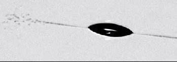
Experimental work by T. Achtzehn, R. Müller, D. Duft and T. Leisner, suggest that when the droplet becomes unstable, it develops a fusiform shape with apices, and later jets of liquid emanate from these tips, as shown in the following figure:
In
this work we want to see if we can justify the formation
of tips by using a simple fluid dynamical model. We would
like to know what happens after the droplet destibilizes,
if there are non-spherical equilibria, and to
describe how the droplet splits into smalles droplets.
Mathematical
formulation
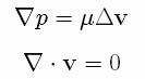
We are going to assume that
the inertia effects are negligible,
so we can describe the fluid
flow with the Stokes equations, valid both inside and
outside the droplet,
with normal stresses given by (using repeated index
summation convention)
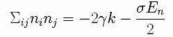
and zero tangential stress
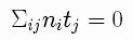
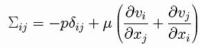
These equations are written using the usual stress tensor
for newtonian fluids
The electric field is
assumed to be electrostatic on the exterior of the drop,
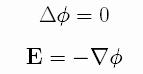
while in the
interior, the electric field is zero, because the
drop is made of a conductor fluid. That means that
the electric potential is a constant at the surface.
The surface evolves because the normal component of
the surface velocity equals the normal
component of the fluid velocity.
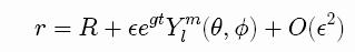
where the perturbing term is a spherical harmonic of
indices l and m, which describe the shape of that
particular mode. By substituting this expression
into the equations of motion and dropping all
quadratic terms we obtain g in terms of the charge
Q, surface tension and the viscosities of the fluid
in the exterior and interior of the drop
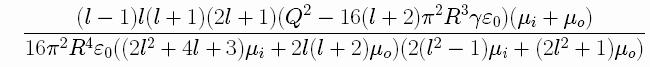
When this quantity is positive, the drop is
unstable, and when is negativ, it is stable. For the
case l=2, it gives the critical charge described
above.
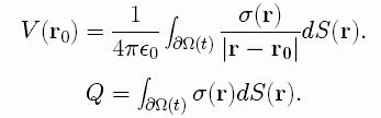
Then we discretize the shape of the droplet with a
series of conical rings (for axi-symmetric
solutions) or with triangles (for general 3D
shapes), and the charge density sigma is solved from
the resulting linear system.
Then we repeat the same procedure for the velocity of the fluid
where we have used the Green functions and the force
per unit area at the surface. At this point we have
the solved the velocity u. Then we move the surface
using this velocity where f is the capillary and
electric force.
As the surface may develop regions of high curvature, we use an adaptive grid, the size of the triangles adapt to the local curvature of the surface: they are smaller in regions of high curvature. We use a combination of techniques: elastic relaxation, addition-deletion of triangles and modified Delaunay triangulation.
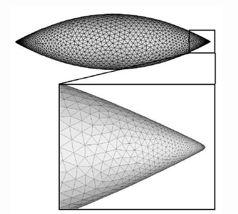
The next figure shows that even if the shape of the droplet is FAR from axisymmetric, still it may develop tips which are locally axisymmetric.
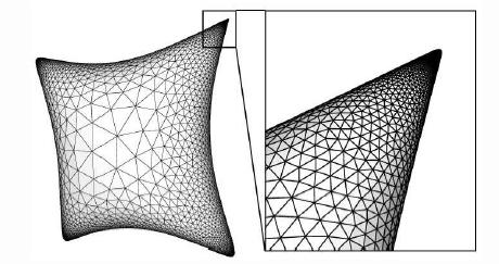
This is anothe example of the same fenomenon, with a droplet with tetrahedral symmetry. The initial shape, not shown in this images, is a sphere perturbed with the mode Y32.
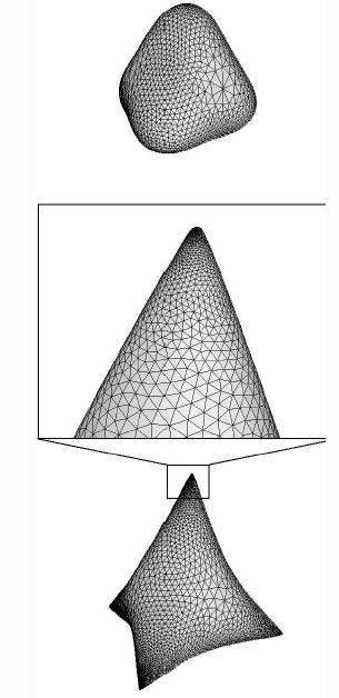
And the corresponding triangulation
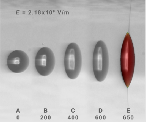
And finally, the result that really matters: the
comparison with the experiments of Beauchamp
(simulation by Orestis Vantzos). The red drop is the
numerical simulation, the grey shapes are
photographs of real drops. In this setup, the drop
is subject to an external electric field.
Linear
stability of the surface
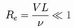
We can get some insight on the stability of the
droplet by looking at the linearized solutions of a
perturbed sphere of radius R Numerical
solution of the initial value problem
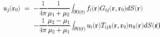
These equations of motion can be solved using the
Boundary Elements Method. First we write the
relation between the electric potential and the
charge density at the surface of the dropThen we repeat the same procedure for the velocity of the fluid
As the surface may develop regions of high curvature, we use an adaptive grid, the size of the triangles adapt to the local curvature of the surface: they are smaller in regions of high curvature. We use a combination of techniques: elastic relaxation, addition-deletion of triangles and modified Delaunay triangulation.
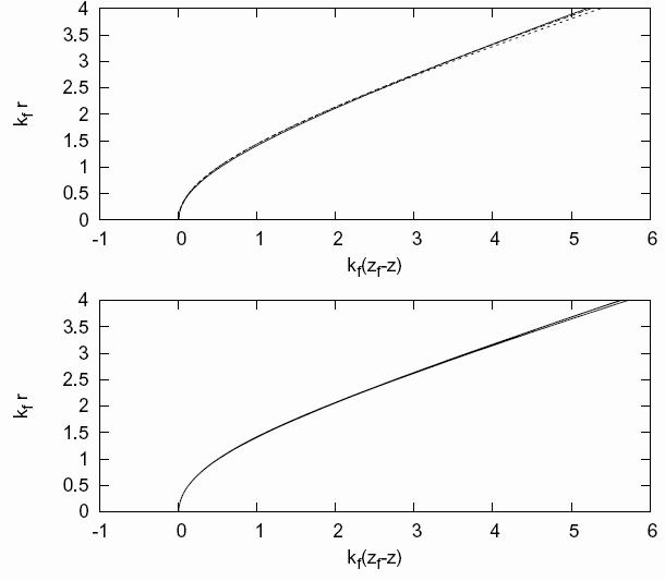
Selfsimilar
dynamics
Now we rescale the above figures with the radius of curvature of the tip, and all the asymptotic profiles lie in the same curve. This is evidence of selfsimilarity. The selfsimilarity exponent is close to 0.5.
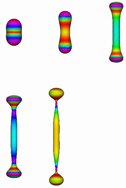
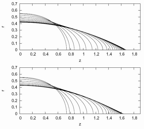
In
the following figures, we perturbed a
sphere with a low amplitude (0.1) mode
Y20, and then we let it evolve, the tips
formation is evident (in the above
figure, the viscosities inside and
outside the drop are equal, in the lower
one, the viscosity outside the droplet
is near zero)
Now we rescale the above figures with the radius of curvature of the tip, and all the asymptotic profiles lie in the same curve. This is evidence of selfsimilarity. The selfsimilarity exponent is close to 0.5.
Non
axisymmetrical simulations
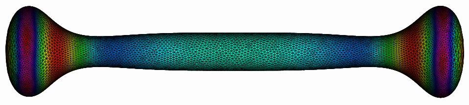
The following image shows that axi-symmetric
droplets develop tips even if we do not restrict the
symmetry of the numerical grid to axial symmetry. It
suggests that the selfsimilar solution is stable
respect to non-axi-symmetric perturbations.Now,
instead of discretizing the droplet with
conical rings, we use triangles, so we
can describe arbitrary three dimensional
shapes (see
the Master's Thesis of Orestis Vantzos
for details).
The next figure shows that even if the shape of the droplet is FAR from axisymmetric, still it may develop tips which are locally axisymmetric.
This is anothe example of the same fenomenon, with a droplet with tetrahedral symmetry. The initial shape, not shown in this images, is a sphere perturbed with the mode Y32.
Finally, not all
droplets develop tips! If the initial charge is
more than twice the critical charge, the droplet
just begins to split without showing tips in the
intermediate steps. This example is also
interesting because it shows that the
axi-symmetry is mantained, however the numerical
grid is not axi-symmetric.
And the corresponding triangulation